Demystifying Vector Embeddings: The Mathematical Backbone of Modern AI

At the heart of every modern AI system—from semantic search engines to Large Language Models (LLMs)—lies a simple but profound mathematical concept: the vector embedding.

Computers cannot natively read words, view images, or understand the intent of a paragraph. They process numbers. To make language computable, we must map discrete tokens (like words or subwords) into a continuous, high-dimensional vector space where geometric distance correlates directly with semantic meaning. This article explores the mathematical foundations of vector embeddings, detailing how tokenized text is mapped to dense coordinate spaces and how AI systems compare them.

---

1. From Sparse to Dense Vectors

Historically, NLP relied on sparse representations like one-hot encoding or Term Frequency-Inverse Document Frequency (TF-IDF).

In a one-hot encoding scheme, every word in a vocabulary of size V is represented by a vector of length V, containing a single 1 and V-1 0s.

Vocabulary: ["cat", "dog", "computer"]
"cat"      -> [1, 0, 0]
"dog"      -> [0, 1, 0]
"computer" -> [0, 0, 1]

This approach has two catastrophic flaws:

1. Dimensionality: A modest vocabulary of 50,000 words requires 50,000-dimensional vectors, leading to massive, memory-inefficient sparse matrices.
2. Semantic Isolation: The dot product of any two distinct one-hot vectors is always zero (\vec{v}_{\text{cat}} \cdot \vec{v}_{\text{dog}} = 0). Mathematically, "cat" is just as distant from "dog" as it is from "computer". No semantic similarity is captured.

Dense embeddings solve this by mapping each word to a dense vector in a much smaller, continuous space (typically d \in [256, 1536] dimensions). In this space, every coordinate is a floating-point number, representing the word's position along a learned semantic axis:

"cat"  -> [-0.12,  0.45,  0.89, ..., -0.03]
"dog"  -> [-0.10,  0.42,  0.81, ..., -0.05]  # Highly similar coordinates
"cpu"  -> [ 0.78, -0.65, -0.21, ...,  0.92]  # Very different coordinates

---

2. Mathematical Similarity Metrics

Once text is projected into a dense vector space \mathbb{R}^d, we can use geometric formulas to measure similarity. The three most common metrics are Cosine Similarity, Dot Product, and Euclidean Distance.

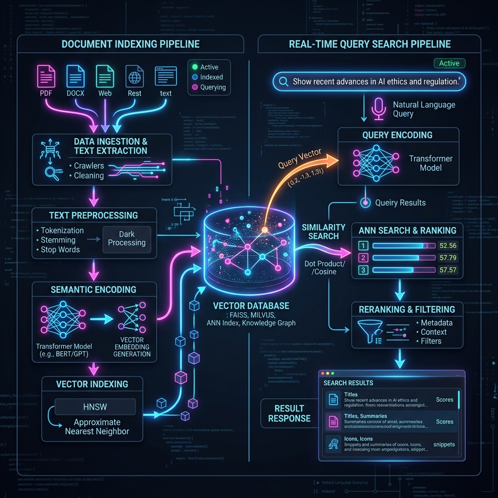Vector Embeddings Math: 3D vector coordinate space mapping word semantic similarity vectors

I. Dot Product

The dot product measures both the direction and magnitude of two vectors.

\text{Dot Product}(\vec{u}, \vec{v}) = \vec{u} \cdot \vec{v} = \sum_{i=1}^{d} u_i v_i

While computationally very fast, it is highly sensitive to vector magnitude. If a document is long or contains highly repeated keywords, its vector magnitude will be larger, artificially inflating the dot product even if the semantic match is weak.

II. Cosine Similarity

Cosine similarity measures only the angle \theta between two vectors, completely ignoring their magnitudes. It represents the cosine of the angle between them:

\text{Cosine Similarity}(\vec{u}, \vec{v}) = \cos(\theta) = \frac{\vec{u} \cdot \vec{v}}{\|\vec{u}\| \|\vec{v}\|} = \frac{\sum_{i=1}^{d} u_i v_i}{\sqrt{\sum_{i=1}^{d} u_i^2} \sqrt{\sum_{i=1}^{d} v_i^2}}

• A value of 1 means the vectors point in the exact same direction (identical semantic alignment).
• A value of 0 means they are orthogonal (uncorrelated).
• A value of -1 means they point in opposite directions (antonyms/opposite meanings).

Note: If vectors are unit-normalized (\|\vec{u}\| = 1), the cosine similarity is mathematically identical to the dot product, which is why many vector databases require embedding normalization.

III. Euclidean Distance (L_2 Norm)

Euclidean distance measures the straight-line distance between two points in high-dimensional space:

d(\vec{u}, \vec{v}) = \|\vec{u} - \vec{v}\|_2 = \sqrt{\sum_{i=1}^{d} (u_i - v_i)^2}

Unlike cosine similarity, lower values indicate higher similarity (closer proximity).

---

3. Python Implementation: Extracting and Measuring Embeddings

Below is a complete implementation using PyTorch and Hugging Face's transformers library to extract embeddings from a transformer model (using Mean Pooling over the token outputs) and computing similarity metrics using NumPy.

import torch
import numpy as np
from transformers import AutoTokenizer, AutoModel

def mean_pooling(model_output, attention_mask):
    """
    Perform mean pooling on token embeddings to get a single sentence representation,
    taking the attention mask into account.
    """
    token_embeddings = model_output[0]  # First element contains all token embeddings
    input_mask_expanded = attention_mask.unsqueeze(-1).expand(token_embeddings.size()).float()
    sum_embeddings = torch.sum(token_embeddings * input_mask_expanded, 1)
    sum_mask = torch.clamp(input_mask_expanded.sum(1), min=1e-9)
    return sum_embeddings / sum_mask

# 1. Compute Geometric Similarity Metrics manually in NumPy
def compute_metrics(v1: np.ndarray, v2: np.ndarray):
    dot_prod = np.dot(v1, v2)
    norm_v1 = np.linalg.norm(v1)
    norm_v2 = np.linalg.norm(v2)
    cosine_sim = dot_prod / (norm_v1 * norm_v2)
    euclidean_dist = np.linalg.norm(v1 - v2)
    
    return {
        "Dot Product": float(dot_prod),
        "Cosine Similarity": float(cosine_sim),
        "Euclidean Distance": float(euclidean_dist)
    }

if __name__ == "__main__":
    # Load a lightweight sentence transformer model
    model_name = "sentence-transformers/all-MiniLM-L6-v2"
    tokenizer = AutoTokenizer.from_pretrained(model_name)
    model = AutoModel.from_pretrained(model_name)

    sentences = [
        "The software engineer compiled the source code.",
        "A programmer wrote the application script.",
        "An organic apple fell from the tall tree."
    ]

    # Tokenize and compute token embeddings
    encoded_input = tokenizer(sentences, padding=True, truncation=True, return_tensors='pt')
    
    with torch.no_grad():
        model_output = model(**encoded_input)
        
    # Get dense sentence embeddings (mean pooled)
    embeddings = mean_pooling(model_output, encoded_input['attention_mask']).numpy()
    
    print(f"Embedding shape: {embeddings.shape} (3 sentences, 384 dimensions each)\n")
    
    emb_engineer = embeddings[0]
    emb_programmer = embeddings[1]
    emb_apple = embeddings[2]
    
    # Calculate similarity metrics
    similar_pair = compute_metrics(emb_engineer, emb_programmer)
    dissimilar_pair = compute_metrics(emb_engineer, emb_apple)
    
    print("Comparing: 'Software engineer code' vs 'Programmer script':")
    for metric, val in similar_pair.items():
        print(f"  {metric}: {val:.4f}")
        
    print("\nComparing: 'Software engineer code' vs 'Organic apple':")
    for metric, val in dissimilar_pair.items():
        print(f"  {metric}: {val:.4f}")

---

4. How Models Learn the Embeddings

Vector embeddings are not arbitrarily assigned; they are learned during training via backpropagation.

In transformer models (like BERT or GPT), embeddings are learned at two levels:

1. Token Embeddings Table: A lookup matrix W_E \in \mathbb{R}^{V \times d} where row i corresponds to the embedding of vocabulary token i. During training, the gradients update this table to position similar characters, subwords, or roots closer together.
2. Contextual Encoders: Unlike static word vectors (like Word2Vec), transformers process words dynamically based on their context. The phrase "bank of a river" and "bank of America" will produce different vectors for the word "bank" because the attention mechanisms compute linear combinations of surrounding tokens' representations.

This contextual density is what allows modern LLMs to disambiguate homonyms and handle structural syntax, cementing embeddings as the essential mathematical conduit between human language and machines.