Indexing the World: How HNSW and Vector Databases Query Millions of Vectors

When querying a relational database, indexing columns with B-Trees ensures lookup complexity remains logarithmic (O(\log N)). However, in high-dimensional vector spaces (e.g., d = 1536), traditional indexing structures break down due to the curse of dimensionality.

If we perform an exact k-Nearest Neighbors (k-NN) search, we must compute the distance between our query vector and every single vector in the database. This linear search (O(N \cdot d)) is computationally prohibitive when N exceeds millions of vectors.

To achieve sub-millisecond latencies, vector databases (like Pinecone, Milvus, and Qdrant) sacrifice 100% precision for speed, utilizing Approximate Nearest Neighbor (ANN) search algorithms. This article breaks down the three core mechanisms of modern vector indexing: HNSW, IVF, and Product Quantization.

---

1. Hierarchical Navigable Small World (HNSW)

HNSW is the gold standard for high-recall graph-based ANN indexing. It is inspired by the Skip List—a probabilistic data structure that allows fast search within a sorted list by maintaining multiple layers of linked lists with varying step sizes.

HNSW translates this multi-layer concept to graphs.

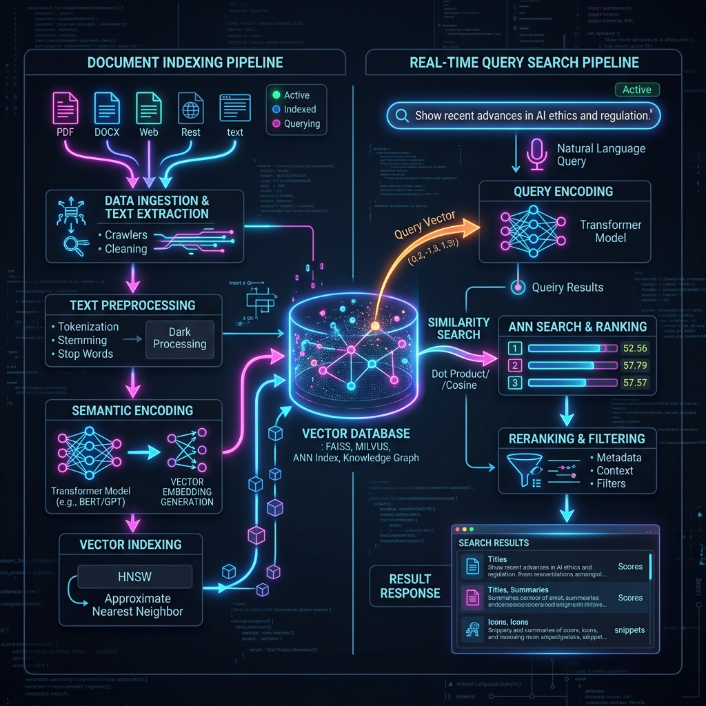Vector Database Indexing HNSW: Hierarchical Navigable Small World graph layers and connected nodes

The Search Process:

1. Start at the Top Layer: The search begins at an entry node in the sparsest layer (Layer L).
2. Greedy Routing: The algorithm computes the distance from the query to all neighbors of the current node. It hops to the neighbor closest to the query.
3. Descent: When no neighbor is closer to the query than the current node, the algorithm drops down to the corresponding node in the next layer (L-1) and repeats the greedy routing.
4. Final Search: This process continues until it reaches Layer 0 (which contains all nodes), where it searches for the k-nearest items using a priority queue.

By utilizing long-range links in upper layers, HNSW quickly navigates to the approximate neighborhood of the query, avoiding local minima.

---

2. Inverted File Index (IVF)

An Inverted File index uses vector clustering to prune the search space. Instead of searching all vectors, it partitions the high-dimensional space into clusters using K-Means clustering.

1. Training Phase: During index creation, the algorithm clusters all database vectors into K centroids. The space is divided into Voronoi cells—regions where any point inside is closer to that cell's centroid than to any other centroid.
2. Indexing Phase: An inverted list (posting list) is created for each centroid, mapping the centroid to all vectors belonging to its Voronoi cell.
3. Query Phase:
   • The query vector's distance to all K centroids is calculated.
   • The algorithm selects the n_{probe} closest centroids.
   • It only computes distances to the vectors contained within those n_{probe} cells.

Increasing n_{probe} increases search recall (accuracy) but also increases search latency, allowing developers to tune the performance trade-off in real-time.

---

3. Product Quantization (PQ)

While HNSW and IVF speed up search, high-dimensional vectors still consume massive amounts of RAM (e.g., 1 million 768-dim float32 vectors require \approx 3 GB of memory). Product Quantization (PQ) is a lossy compression technique that reduces memory footprint by up to 95%.

PQ decomposes the vector space into a Cartesian product of lower-dimensional subspaces:

1. A 1024-dimension vector is split into M = 8 sub-vectors of size 128.
2. For each sub-vector space, K-Means clustering is run to find K = 256 centroids. These centroids are stored in a Codebook.
3. Since K=256, each centroid index can be represented by a single byte (2^8 = 256).
4. The original 1024-dimension vector of float32 (4096 bytes) is compressed into a sequence of M=8 bytes representing the closest centroid index in each sub-space.

When searching, Asymmetric Distance Computation (ADC) is used. The query vector is kept uncompressed, and its distance is calculated directly against the codebook centroid values, avoiding slow decompression cycles.

---

4. Benchmark: FAISS Indexing in Python

The following Python script uses Facebook AI Similarity Search (faiss) to build and compare three indexing approaches: IndexFlatL2 (exact linear search), IndexIVFFlat (clustering), and IndexHNSWFlat.

import time
import numpy as np
import faiss

# Set random seed for reproducibility
np.random.seed(42)

# Configuration
num_vectors = 100000     # 100k vectors in the database
dimension = 128          # Vector dimension
num_queries = 100        # Number of query requests
k = 10                  # Get top 10 nearest neighbors

# Generate synthetic dataset and queries
print("Generating synthetic data...")
db_vectors = np.random.random((num_vectors, dimension)).astype('float32')
query_vectors = np.random.random((num_queries, dimension)).astype('float32')

# ----------------------------------------------------
# 1. FLAT INDEX (Exact Search - Baseline)
# ----------------------------------------------------
print("\n--- Flat Index (Exact K-NN) ---")
flat_index = faiss.IndexFlatL2(dimension)
flat_index.add(db_vectors)

start = time.time()
distances_flat, indices_flat = flat_index.search(query_vectors, k)
flat_time = (time.time() - start) * 1000
print(f"Query latency (100 queries): {flat_time:.2f} ms")

# ----------------------------------------------------
# 2. IVF INDEX (Approximate Search via Clustering)
# ----------------------------------------------------
print("\n--- IVF Index (Approximate) ---")
quantizer = faiss.IndexFlatL2(dimension)  # coarse quantizer
nlist = 100                              # Number of clusters
ivf_index = faiss.IndexIVFFlat(quantizer, dimension, nlist, faiss.METRIC_L2)

# IVF requires training to calculate cluster centroids
ivf_index.train(db_vectors)
ivf_index.add(db_vectors)
ivf_index.nprobe = 10                    # Number of clusters to search

start = time.time()
distances_ivf, indices_ivf = ivf_index.search(query_vectors, k)
ivf_time = (time.time() - start) * 1000

# Compute recall against exact flat search
recall_ivf = np.mean([len(np.intersect1d(indices_flat[i], indices_ivf[i])) / k for i in range(num_queries)])
print(f"Query latency (100 queries): {ivf_time:.2f} ms")
print(f"Recall (Accuracy compared to Flat): {recall_ivf * 100:.2f}%")

# ----------------------------------------------------
# 3. HNSW INDEX (Approximate Search via Graphs)
# ----------------------------------------------------
print("\n--- HNSW Index (Approximate) ---")
# M = number of bi-directional links per node
hnsw_index = faiss.IndexHNSWFlat(dimension, 32)
hnsw_index.hnsw.efSearch = 64  # Search expansion factor

hnsw_index.add(db_vectors)

start = time.time()
distances_hnsw, indices_hnsw = hnsw_index.search(query_vectors, k)
hnsw_time = (time.time() - start) * 1000

recall_hnsw = np.mean([len(np.intersect1d(indices_flat[i], indices_hnsw[i])) / k for i in range(num_queries)])
print(f"Query latency (100 queries): {hnsw_time:.2f} ms")
print(f"Recall (Accuracy compared to Flat): {recall_hnsw * 100:.2f}%")

---

5. Architectural Trade-offs

Choosing the right index depends heavily on application constraints:

| Index Type | Search Speed | Memory Footprint | Recall (Accuracy) | Build/Index Time | | :--- | :--- | :--- | :--- | :--- | | Flat | Extremely Slow (O(N)) | Medium (Raw Vectors) | 100% | Instant (O(1)) | | HNSW | Blazing Fast (O(\log N)) | Very High (Graph overhead) | 95-99% | Slow | | IVF | Fast | Medium | 80-95% | Medium (Requires training) | | IVF+PQ | Very Fast | Extremely Low (Compressed) | 70-90% | Slow |

For latency-critical applications with large budgets, HNSW offers unmatched recall and speed at the cost of high RAM consumption. When scaling to billions of vectors on a budget, combining IVF with Product Quantization (IVF-PQ) is mandatory to fit the data within manageable memory boundaries.