The Transformer Architecture: Self-Attention Under the Hood
 By Bishwambhar Sen
Before the introduction of the Transformer architecture in 2017, Recurrent Neural Networks (RNNs) and Long Short-Term Memory networks (LSTMs) ruled sequential data processing. However, they had a fundamental limitation: they process tokens sequentially, one step at a time. This sequence-dependent processing makes parallelization impossible, limiting training speed on modern GPUs.
Transformers solved this with the Self-Attention mechanism. By looking at all words in a sequence simultaneously and calculating how much attention to pay to each, the Transformer achieved state-of-the-art results while enabling massive parallelization.
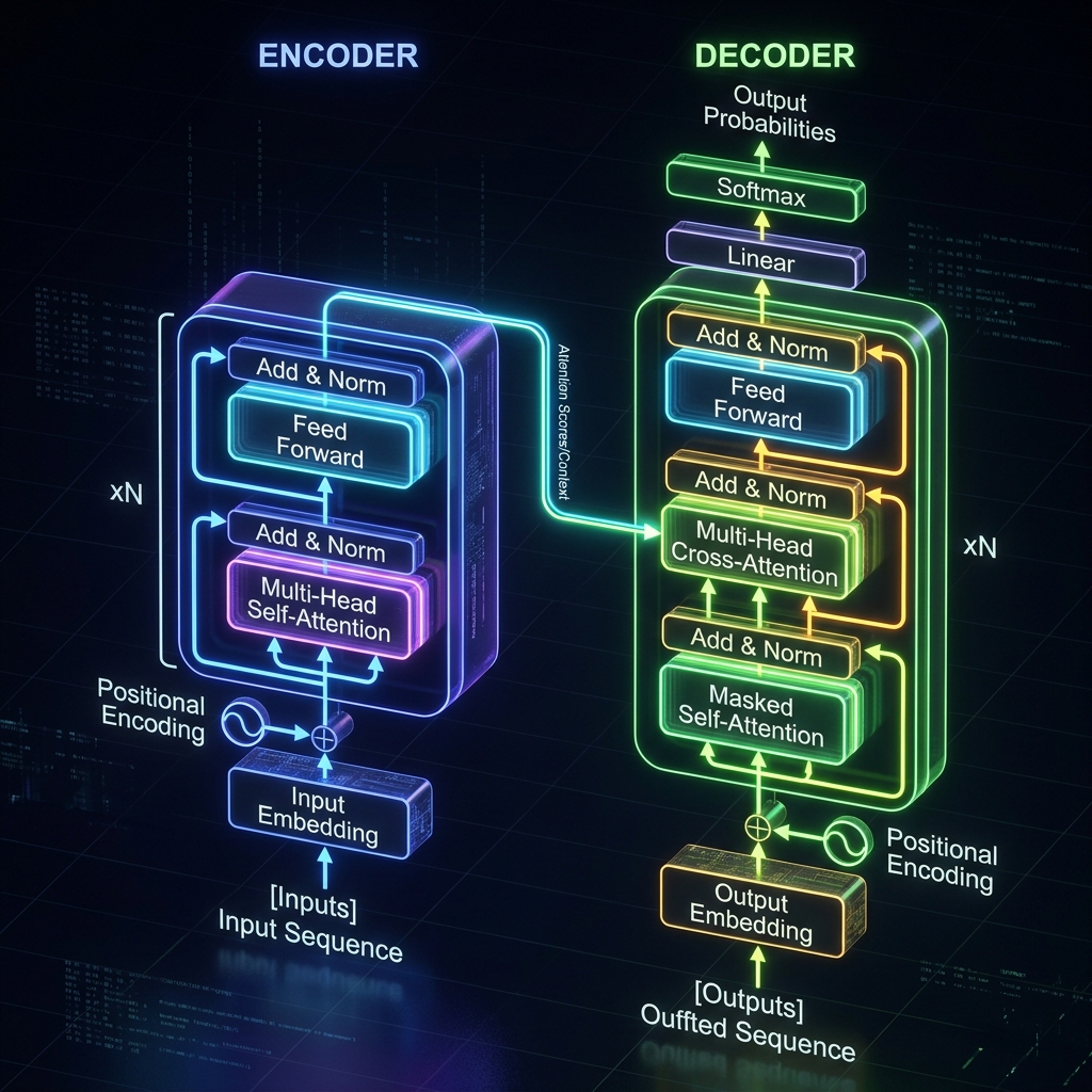 Transformer Architecture Breakdown: 3D block diagram of Transformer encoder-decoder architecture
1. The Core Idea: Query, Key, and Value
To understand self-attention, think of it like searching a database:
- A Query (
Q) represents the token currently being processed (what we are looking for). - A Key (
K) represents all the tokens in the sequence (what we compare the query against). - A Value (
V) represents the actual content of the tokens (what we retrieve).
For each input token vector x, we project it into Query, Key, and Value vectors using weight matrices W^Q, W^K, and W^V:
q = x W^Q, \quad k = x W^K, \quad v = x W^V
2. Scaled Dot-Product Attention
The similarity between a Query and a Key is calculated using their dot product. Higher values indicate that the tokens are highly related. The mathematical formulation of Scaled Dot-Product Attention is:
\text{Attention}(Q, K, V) = \text{softmax}\left(\frac{Q K^T}{\sqrt{d_k}}\right) V
Where:
Q, K, Vare the query, key, and value matrices.d_kis the dimension of the key vectors.\sqrt{d_k}is the scaling factor.
Why do we scale by \sqrt{d_k}?
For large values of d_k, the dot product grows large in magnitude. This pushes the softmax function into regions with extremely small gradients (vanishing gradients). Dividing by \sqrt{d_k} stabilizes training by keeping the values in a range where softmax has active gradients.
       Q Matrix       K^T Matrix          Attention Map           V Matrix       Final Output
      [  q1  ]   x   [ k1  k2 ]   --->   [ s11  s12 ]   x   [  v1  ]   --->   [   o1   ]
      [  q2  ]                           [ s21  s22 ]       [  v2  ]          [   o2   ]
3. Multi-Head Attention
Instead of performing self-attention once, the Transformer splits the queries, keys, and values into multiple subspaces, allowing the model to attend to information from different representation subspaces at different positions simultaneously.
The formulas for Multi-Head Attention are:
\text{MultiHead}(Q, K, V) = \text{Concat}(\text{head}_1, \dots, \text{head}_h) W^O
\text{head}_i = \text{Attention}(Q W_i^Q, K W_i^K, V W_i^V)
Where the projection matrices are:
W_i^Q \in \mathbb{R}^{d_{model} \times d_k}W_i^K \in \mathbb{R}^{d_{model} \times d_k}W_i^V \in \mathbb{R}^{d_{model} \times d_v}W^O \in \mathbb{R}^{h d_v \times d_{model}}
4. PyTorch Implementation of Multi-Head Attention
Let's write a complete, raw implementation of Multi-Head Attention in PyTorch using tensor reshaping operations.
import torch
import torch.nn as nn
import math

class MultiHeadAttention(nn.Module):
    def __init__(self, d_model, num_heads):
        super(MultiHeadAttention, self).__init__()
        assert d_model % num_heads == 0, "d_model must be divisible by num_heads"

        self.d_model = d_model
        self.num_heads = num_heads
        self.d_k = d_model // num_heads

        # Projection matrices
        self.w_q = nn.Linear(d_model, d_model)
        self.w_k = nn.Linear(d_model, d_model)
        self.w_v = nn.Linear(d_model, d_model)
        self.w_o = nn.Linear(d_model, d_model)

    def forward(self, q, k, v, mask=None):
        batch_size = q.size(0)

        # 1. Project inputs and split into heads
        # Shape changes: (batch, seq_len, d_model) -> (batch, seq_len, num_heads, d_k) -> transpose to (batch, num_heads, seq_len, d_k)
        Q = self.w_q(q).view(batch_size, -1, self.num_heads, self.d_k).transpose(1, 2)
        K = self.w_k(k).view(batch_size, -1, self.num_heads, self.d_k).transpose(1, 2)
        V = self.w_v(v).view(batch_size, -1, self.num_heads, self.d_k).transpose(1, 2)

        # 2. Compute Scaled Dot-Product Attention scores
        # (batch, num_heads, seq_len, d_k) x (batch, num_heads, d_k, seq_len) -> (batch, num_heads, seq_len, seq_len)
        scores = torch.matmul(Q, K.transpose(-2, -1)) / math.sqrt(self.d_k)

        if mask is not None:
            # Mask out invalid padding or future tokens (causal masking)
            scores = scores.masked_fill(mask == 0, -1e9)

        attention_weights = torch.softmax(scores, dim=-1)

        # 3. Multiply attention weights by values
        # (batch, num_heads, seq_len, seq_len) x (batch, num_heads, seq_len, d_k) -> (batch, num_heads, seq_len, d_k)
        context = torch.matmul(attention_weights, V)

        # 4. Concatenate heads back and apply output projection
        # Transpose back: (batch, num_heads, seq_len, d_k) -> (batch, seq_len, num_heads, d_k)
        context = context.transpose(1, 2).contiguous().view(batch_size, -1, self.d_model)

        return self.w_o(context)

# Testing the implementation
batch_size, seq_len, d_model, num_heads = 2, 8, 64, 4
qkv_tensor = torch.randn(batch_size, seq_len, d_model)

mha = MultiHeadAttention(d_model=d_model, num_heads=num_heads)
out = mha(qkv_tensor, qkv_tensor, qkv_tensor)
print("Output tensor shape:", out.shape)  # Expected: [2, 8, 64]
5. Positional Encoding
Because the Self-Attention mechanism computes attention across all tokens in parallel, it is completely invariant to sequence order. In other words, the sequence "the cat ate the fish" and "the fish ate the cat" would result in identical self-attention representations.
To restore sequence order, we inject Positional Encodings into the input token embeddings. These are vectors containing unique periodic signals based on sine and cosine functions:
PE_{(pos, 2i)} = \sin\left(\frac{pos}{10000^{2i/d_{model}}}\right)
PE_{(pos, 2i+1)} = \cos\left(\frac{pos}{10000^{2i/d_{model}}}\right)
This mathematical formulation gives the model a unique, geometry-based positional coordinate for every token.
What the 2017 Design Got Wrong
It's easy to read the original architecture as settled, but several pieces of it have been quietly replaced in every model you actually use, and knowing which is the difference between understanding Transformers and understanding the 2017 paper.
Sinusoidal positional encoding is the clearest example. The claim that it extrapolates to unseen sequence lengths turned out not to hold in practice — models trained at 512 tokens degrade badly past that regardless of the elegant periodic construction. Contemporary models use RoPE, which rotates Q and K by a position-dependent angle so attention scores depend on relative distance rather than absolute index, and that change is most of why long-context models work at all. Likewise, the masked_fill(mask == 0, -1e9) in the implementation above is the standard idiom and it is a bug waiting to happen in fp16, where -1e9 overflows to -inf and a fully-masked row yields NaN after softmax. Use torch.finfo(scores.dtype).min.
The deeper limitation is the one the parallelism buys: that seq_len × seq_len score matrix is quadratic in memory as well as compute. Doubling context quadruples the attention cost, which is the entire reason context windows were stuck in the low thousands for years and why FlashAttention — which never materialises the full matrix, tiling the computation through SRAM instead — was such a significant result. In production you should essentially never write the forward pass above; call torch.nn.functional.scaled_dot_product_attention and get the fused kernel. Write it by hand once, to know what the kernel is doing, then delete it.
If you want one intuition to carry forward: attention is a soft, differentiable dictionary lookup, and nearly every architectural advance since 2017 has been an attempt to make that lookup cheaper without making it dumber. Multi-Query and Grouped-Query Attention shrink the K and V heads to cut KV-cache memory. Sliding-window attention restricts which keys a query may see. Mixture-of-Experts leaves attention alone and sparsifies the feed-forward layers instead. Each is a different answer to the same question, and each trades away something the full quadratic version had.