Understanding Activation Functions: ReLU, Sigmoid, and Beyond | FromZero2AI Blog

Without activation functions, even the most massive deep learning models would collapse into simple linear models. Activation functions determine whether a neuron should fire and determine the strength of its output signals.

In this guide, we will analyze why activation functions are necessary, examine classic and modern variants (Sigmoid, Tanh, ReLU, and Leaky ReLU), evaluate their mathematical derivatives, and implement them in Python.

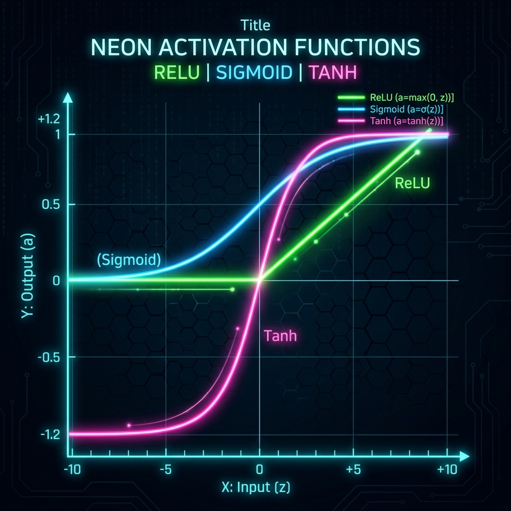Activation Functions Guide: Graph showing curves of ReLU, Sigmoid, and Tanh activation functions Activation Functions Guide: Graph showing curves of ReLU, Sigmoid, and Tanh activation functions

Why Do We Need Activation Functions?

A neural network layer computes a weighted sum of inputs and adds a bias:

z = \sum w_i x_i + b

If we stack multiple layers without applying a non-linear transformation, the composition of these layers remains linear. Let's see this mathematically. If layer 1 is y_1 = W_1 X + b_1 and layer 2 is y_2 = W_2 y_1 + b_2, then:

y_2 = W_2 (W_1 X + b_1) + b_2 = (W_2 W_1) X + (W_2 b_1 + b_2)

Since the product of two matrices (W_2 W_1) is just another matrix W_{new} and (W_2 b_1 + b_2) is a new bias vector b_{new}, the entire network collapses into a single-layer linear model.

Non-linear activation functions allow neural networks to approximate complex, non-linear decision boundaries, enabling them to solve problems like image classification and language modeling.

Classical Activation Functions

1. The Sigmoid Function

The Sigmoid function maps real-valued numbers into a probability range between 0 and 1.

\sigma(x) = \frac{1}{1 + e^{-x}}

Pros:

Smooth gradient curve.
Perfect for output layers of binary classifiers.

Cons (The Vanishing Gradient Problem):

For very large positive or negative inputs, the slope of the sigmoid function becomes nearly flat (its derivative approaches 0). During backpropagation, these tiny gradients are multiplied through layers, preventing the network weights from updating. This is known as the vanishing gradient problem.

2. The Tanh (Hyperbolic Tangent) Function

Tanh is a mathematically shifted version of the sigmoid, mapping inputs to a range between -1 and 1.

\tanh(x) = \frac{e^x - e^{-x}}{e^x + e^{-x}}

Pros:

Zero-centered: Output values average close to zero, which makes optimization for subsequent layers more stable.

Cons:

Still suffers from the vanishing gradient problem at its extremes.

The Modern Standards

3. ReLU (Rectified Linear Unit)

Introduced to overcome the vanishing gradient problem, ReLU is the most widely used activation function in deep learning.

f(x) = \max(0, x)

Pros:

Computational Efficiency: Calculating a maximum is much faster than computing exponentials.
Sparsity: Outputs exactly zero for negative inputs, which means only active neurons participate in computations.
No Vanishing Gradient: The derivative is a constant 1 for all positive inputs.

Cons (The Dying ReLU Problem):

If a neuron receives inputs that cause it to output negative values, the gradient becomes exactly 0. Once a neuron is stuck in this state, it will never update its weights during backpropagation, becoming "dead."

4. Leaky ReLU

To address the dying ReLU problem, Leaky ReLU introduces a small slope (usually 0.01) for negative inputs.

f(x) = \max(\alpha x, x) \quad \text{where } \alpha = 0.01

This ensures that even for negative values, a small gradient flows back through the network.

Mathematical Summary of Activation Derivatives

During backpropagation, we need the derivatives of the activation functions. Here is the mathematical comparison:

| Activation | Formula | Range | Derivative | | :--- | :--- | :--- | :--- | | Sigmoid | \frac{1}{1 + e^{-x}} | (0, 1) | \sigma(x)(1 - \sigma(x)) | | Tanh | \frac{e^x - e^{-x}}{e^x + e^{-x}} | (-1, 1) | 1 - \tanh^2(x) | | ReLU | \max(0, x) | [0, \infty) | 1 if x > 0 else 0 | | Leaky ReLU| \max(\alpha x, x) | (-\infty, \infty)| 1 if x > 0 else \alpha |

Python / NumPy Implementation

Let's implement these activation functions and their derivatives using NumPy:

import numpy as np

def sigmoid(x):
    return 1 / (1 + np.exp(-x))

def sigmoid_derivative(x):
    s = sigmoid(x)
    return s * (1 - s)

def tanh(x):
    return np.tanh(x)

def tanh_derivative(x):
    return 1.0 - np.tanh(x) ** 2

def relu(x):
    return np.maximum(0, x)

def relu_derivative(x):
    # Returns 1 for positive inputs, 0 otherwise
    return np.where(x > 0, 1.0, 0.0)

def leaky_relu(x, alpha=0.01):
    return np.where(x > 0, x, x * alpha)

def leaky_relu_derivative(x, alpha=0.01):
    return np.where(x > 0, 1.0, alpha)

# Test the implementations
test_inputs = np.array([-2.0, -0.5, 0.0, 1.0, 3.0])

print("Raw Inputs:", test_inputs)
print("ReLU Output:", relu(test_inputs))
print("ReLU Derivative:", relu_derivative(test_inputs))
print("Leaky ReLU Derivative:", leaky_relu_derivative(test_inputs))

Conclusion

Choosing the right activation function directly impacts training speed and model stability. For hidden layers, ReLU or Leaky ReLU are the default choices to prevent vanishing gradients and minimize computation. For output layers, Sigmoid is used for binary classification, and Softmax (a multi-class generalization of sigmoid) is used for multi-class classification problems.